
Autophaser Guide
1 Introduction
Autophaser is a software package intended to automate the production of absorption mode FT-ICR MS spectra. Currently the package is capable or reading both Bruker .d data-files and AMOLF .awm spectra.
The system can output Bruker XMass style data-files which can be re-opened in DataAnalysis for normal processing.
Autophaser is designed to run on a 64bit computer. The development machine is a Dell Optiplex 390, Core i5 processor, 8Gb memory, running Windows 7.
2 User interface
The Autophaser user interface is shown in Figure 1. There are two major tab groups: the control tabs (left hand side of the user interface) and the display tabs (right hand side of the user interface).
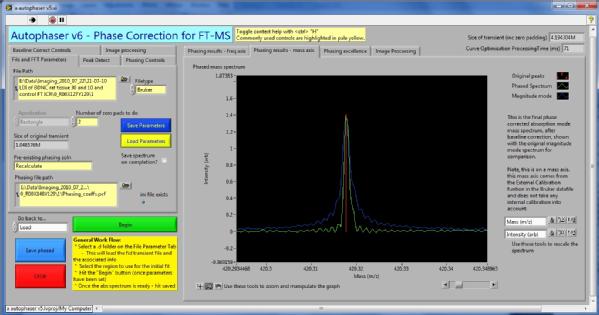
Figure 1 – The Autophaser user interface.
The control tabs are:
- File and FFT Parameters
- Peak Detect
- Phasing Controls
- Baseline Correct Controls
The display tabs are:
- Phasing results – freq axis
- Phasing results - mass axis
- Phasing excellence
All controls and indicators are labelled. Additional contextual help can be displayed by typing <Ctrl>H and pointing at a control or indicator. <Ctrl>H can then also be used to toggle contextual help off again.
2.1 Loading files
To load files for phasing, use the browse button next to the "File path" control on the "File and FFT parameters" control tab. This will open a file dialog box.
To select a bruker .d file, open the .d file (it is actually a folder) and then use the "Select current folder" at the bottom of the file dialog box.
To select a .awm file, select the file as normal - .awm files are actual files and not folders.
Use the "Filetype" control on the "File and FFT parameters" control tab to select which type of file you wish to process.
3 Basic Operation
- When Autophaser is loaded, it will run automatically. User the “File Path” control to navigate to the .d folder or .awm file you wish to phase.
- Note - Bruker .d data-files are actually Windows folders, so in order to select a .d folder for phasing, use the browse button and navigate until the .d folder is open; then click the “select current folder” button at the bottom of the file dialog.
- Support for IonSpec files is only at the prototype stage.
- Check the settings of all the other controls on the Control Tabs.
- In particular, check the “Number of zero pads to do” – it can take a long time to phase a very large spectrum and every zero pad doubles the length.
- Hit the “Begin” button.
- This will be flashing.
- Autophaser will load the file and begin the peak detection process.
- In the Peak Detection window, make sure that mass spectral peaks and not noise or side band peaks are being detected.
- Use the “K Hi density” (akin to a threshold) and “Peak width” controls in particular.
- These are also on the “peak detect” control tab on the main UI.
- Use the “K Hi density” (akin to a threshold) and “Peak width” controls in particular.
- When you are happy that you are correctly able to detect the right peaks, click “Accept peak definitions”
- Autophaser will move onto the Fit Initial Region window (providing Recalculate mode is selected – check the Pre-exiting phasing soln control.)
- The Auto search function will try to find a phase correction function in your initial region
- If there were not enough detected peaks in the intial region, you will be prompted to identify another region. At low mass, only short regions can be used but at high mass, initial regions can get much larger.
- If the initial guess function is good then the Rephased Re spectrum in the “Spectrum” graph indicator will have all the peaks positive – in this case, click the green “Accept calibration function” button to continue.
- If not – use the Fit Initial Region section of this guide to investigate the reason why.
- Autophaser will then use one of its tuning methods to extend this initial phase correction function out to cover the complete spectrum and will generate absorption mode spectra on both a frequency and mass axis.
- Use the “Baseline Correct Controls” tab to fine-tune the baseline you wish to correct
- Look for the red line on the “Phasing results – freq axis” display tab
- The corrected absorption mode spectrum will appear in the “Phasing results – mass axis” tab.
- Hit the “Save phased” and save the absorption mode spectrum to an XMASS format file for analysis in Bruker DataAnalysis.
- Hit “Stop” to finish Autophaser.
4 Workflow Options
Autophaser has three standard workflows for processing single FT-ICR spectra.
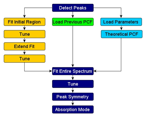
Figure 2: The three different workflows in Autophaser 5.1.
The choice of which workflow to use will depend on the data file which is to be processed. The workflow (mode) to be used is set using the "Pre-existing phasing soln" control on the File and FFT Controls tab.
4.1 Load Previous PCF - Green Channel
If you have previously phase corrected the current or a similar file, then Autphaser will have saved the phase correction function parameters in a .pcf file in the directory. You can use this previously saved phase correction function as a basis for attempting to phase or re-phase the current file. If this option is selected then Autophaser will attempt to phase correct peaks across the entire spectrum using this phase correction function and then optimise the resulting absorption mode spectrum. Either the "Use previous for this file" or "Use previous for another file" modes will follow this work flow.
If "Use previous for another file" is selected, then you must identify which pcf file to use in the filepath control beneath.
4.2 Theoretical PCF - Light Blue Channel
In the more modern versions of the Bruker software (post 2010), the system saves certain parameters about the spectral collection which can be used to estimate the phase correction function. This can also be used as the basis for phasing the spectrum. If the "Use ab inito values" option is selected then Autophaser will attempt to phase correct peaks across the entire spectrum using this estimated phase correction function and then optimise the resulting absorption mode spectrum.
This mode will normally be successful, but we have seen exmaples of datafiles where the estimation of the phase correction function is not sufficiently close to allow the tuning algorithm to work. We believe this may be due to the ion oscillation frequencies shifting slightly during excitation. In the event that this approach does not work, try one of the other methods.
4.3 Create New PCF - Yellow Channel
It is possible to generate a phase correction function with no prior knowledge. In this work flow, the system will take a user designated Initial Region, and attempt to produce a phse correction function for that region by a brute force trial and error method (see Section 9).
This initial phase correction function can then be extended to cover the complete spectrum.
The "Recalculate" mode will follow this workflow and the Basic Operation, Section 3, above will explain the processes.
5 Peak detection
Good peak detection is key to getting reliable phase correction. Autophaser only uses the peak apex values of frequency and phase in order to produce the phase correction function. If your peak detection parameters allow the system to detect too many noise or side band peaks as well as the real peaks, then the system may not be able to solve for the phase correction function. So, it is worthwhile getting peak detection working well.
Peak detection in Autophaser does not use a simple linear threshold method. Instead, the system will identify peak regions as anomalies which are above the local noise environment. So, the system first analyses the noise and uses this to determine if any point in the spectrum is likely to be part of a peak. Points are determined to be likely to be anomalous (i.e. possibly in a peak) if the difference between their intensity and that of the previous noise points is much larger than would be normal for the noise. If you have a certain number of contiguous points which are all considered anomalously high, then that becomes a detected peak.
See also the Peak Detect Section.
6 Graph Interfaces
Labview graphs all have the same core look and controls. The placement may vary, but the operation does not.
6.1 Graph tools
- Cursor Tool – Select this tool to drag cursors (if present)
- Zoom Tools– Click here to select one of the graph zoom tools
- Use the rescale buttons on the Scale controls to rescale graph
- Grab Tool – Select to grab the graph to reposition the field of view
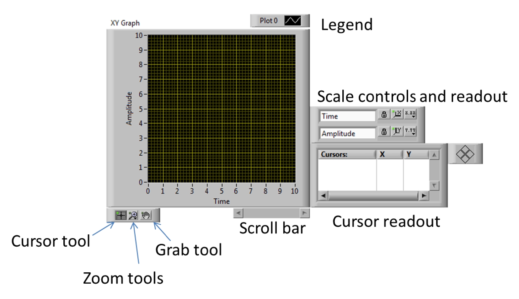
Figure 3: The standard graph tools in LabVIEW.
You can export the visible portion of any graph to Excel or the clipboard but right clicking ont he graph and selecting the Export data option. This functionality can be very useful for data plotting purposes.
6.2 Scroll bar
Use this to scroll along the X direction
6.3 Cursor Readout
The positions of any cursors are displayed here. Right click on the title of any cursor to further options, such as “Bring to center” or “Go to cursor”
6.4 Scale Controls
- Title – the title of the cursor
- Lock tool – turn autoscale on and off
- Fit to – re-fit to either the X or Y axis
- Scale format – control format, precision and mapping mode.
7 Control Tabs
7.1 File and FFT Parameters
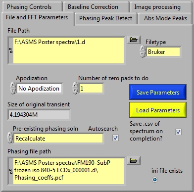
Figure 4: File and FFT parameter controls.
- File path– Use the browse button to navigate to the file/folder of choice.
- Note - Bruker .d data-files are actually Windows folders, so in order to select a .d folder for phasing, use the browse button and navigate until the .d folder is open; then click the “select current folder” button at the bottom of the file dialog.
- File type to load – select either Bruker (.d) or AMOLF (.awm) files.
- Apodization - Choose a type of apodization to apply to the transient before zeropadding and Fourier Transformation.
- NOTE - Absorption mode spectra should normally be generated from un-apodized data or Half Hanning apodized.
- Number of zero pads to do– each zero pad operation doubles the length of the transient by adding extra zeros.
- Normally, this should be set to 1 or 2.
- Beware using high numbers as this will generate a very large memory footprint.
- Pre-existing phasing solution– choose between:
- Recalculate – uses the full programme to attempt to generate a new phase correction function by brute force fitting to a small initial region and extending up to the complete spectrum. This is the normal mode of operation.
- Use previous for this file – Simply apply the phase correction function which has already been solved for this file.
- Use previous for another file - if, instead of working up the phase solution for a spectrum in the normal way, it will be simpler to use the solution for a similar file which has already been phased and saved, select this option. Autophaser will use its normal tuning function to attempt to overcome any changes in the phase correction function which might be a result of, for example, space charge or image charge.
- Use previous no tuning – as above, except that the phase correction function will not be tuned. This is to illustrate the importance of tuning only.
- Use ab initio values – this mode causes Autophaser to generate an initial phase correction function based on information about the excitation sweep and delay times that were used when the spectrum was collected. This information can only be read from certain versions of Bruker data-files. The phase correction function generated in this way must be optimised (this will be done automatically) to produce an absorption mode spectrum. We have found, in practice, that this approach is generally, but not universally, successful. Sometimes, the frequency shift during exciation is too great. If this mode does not work – try using Recalculate mode instead.
- Autosearch - the programme will attempt to find an initial region (only applicable of "Recalculate" mode is selected). When this mode is selected, the user does not have to define the initial region which will be used to generate a candidate phase correction fuction, which will be extended and optimised over the complete spectrum to produce a complete phase correction function. Instead, the system will search through the spectrum to find the region with the greatest peak density and will use this as the initial region. In general, in order for this funtion to work, there must be sufficient peak density within the spectrum and there should be sufficient resolution to resolve all peaks across the complete mass range within the sample. If the system cannot find a region to use, it will generate a pop-up dialogue box - normally this will be because there is not sufficient peak density for the system to detect a region usig its automatic algorithm. In this case, it will prompt the user to define the intial region of their choice. This function is in development and may not provide final functionality yet, although inital testing has sugested that it can be quite successful. Simply uncheck this box if unwanted behaviour results.
- Phasing file path – Only used if “Use previous for another file” of “Use previous no tuning” modes hav been selected
- The file path of the file from which Autophaser should upload the phase correction function.
- Save spectrum on completion – turn this on to cause the system to save the spectrum to a series of csv files (detected peaks, absorption mode spectrum, magnitude mode spectrum) which can be used for producing figures etc.
- Ini file exists – this output will determine if the system was able to identify the Autophaser ini file which is used to save the state of the programme from use to use.
7.2 Peak Detect
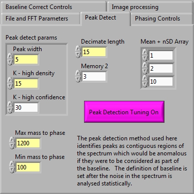
Figure 5: Peak Detect controls.
Autophaser identifies peak regions of the spectrum by a method which is a development of the techniques described by Williams et al. and Friedman1, 2.
The spectrum is decimated into sections of a length selected by the user (Decimate length - usually between 50 and 500 points, depending on the spectrum); the median value of each section is taken. The difference between the median value of each region is compared to that of the next, and the mean (m) and standard deviation (SD) of those differences is calculated. Each section is classified as being accepted as being part of a putative baseline if the difference between the median value of that decimated region and the next is less than (m × n.SD), where n is an integer value set by the user (Mean + nSD Array). The accepted points are passed through a Savitsky-Golay filter3 to produce a smoothed putative baseline for the decimated spectrum (Memory 2 = length of S-G range). To allow for the various changes in scale for the peaks, noise and baseline deviation in the uncorrected absorption mode spectrum, three different values of n are used, and the putative baselines of all three values of n are taken onto the next stage: this step is analogous to the variable span concept of Friedman’s supersmoother. Linear interpolation of these decimated arrays is used to generate three arrays (B1, B2, and B3), which provide a putative baseline value for every point in the original spectrum.
The spectrum is statistically analysed in order to determine the standard deviation (SDs) of the intensity difference between any point and the next point. Points in the original spectrum (Si) are classed as being potentially part of a peak if they are greater than the minimum of the three putative baseline predictions for that point, plus n ×SDs (Eqn(1)):
|
|
|
(1) |
Where, K, K Threshold and K Multiplier are controlled by the user. The point is only confirmed as being part of peak if there are at least a certain number of contiguous points in the same peak (Peak width).
K Threshold and K Multiplier allow the user more control over the peak threshold used. Both effectively raise the threshold, but the former will do this linearly and the latter multiplactively. The latter option is particularly useful if the spectrum contains a signal to noise level which varies strongly across the spectrum.
Other controls:
- Max mass to phase– the maximum mass to phase
- Defines the upper mass limit of the absorption mode spectrum
- Min mass to phase– the minimum mass to phase
- Defines the lower mass limit of the absorption mode spectrum
- Skip user tuning – turn this function on if you are phasing a series of files with similar peak detection requirements.
7.3 Phasing Controls

Figure 6: Phasing controls.
For the initial brute force fitting, you must select an initial region to fit to - if the Autosearch finction canot find one automatically. This region should have a good peak density. The length of the fitting region can be controlled. As a general rule, of the start mass of the initial region is low, the region should be short. Conversely, if the start mass if higher, the region can be longer. The exact values will vary according to the mass spectrometer concerned (mainly on the magnetic field and the excitation ramp rate). On our 12T Solarix system, with standard ramp rates, the following values have been useful guides:
|
Start mass of initial fit region (Da) |
Approx Length (Da) |
|
200 |
7 |
|
300 |
12 |
|
400 |
25 |
|
450 |
30 |
|
500 |
35 |
|
600 |
50 |
|
1000 |
100-250 |
The final fit algorithm button is used to toggle between the two available tuning functions; the iterative “Wobbler” function and the newer genetic Algorithm (GA). The GA method is faster and is likely to be the more useful.
6.3.1 Genetic Algorithm Tuning
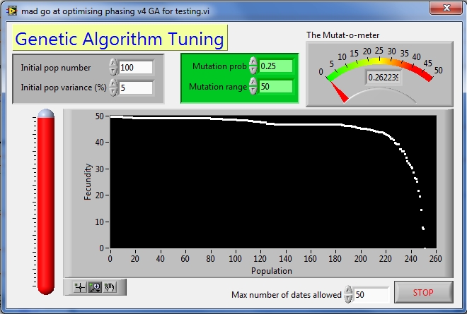
Figure 7: GA tuning user interface.
The GA tuning method is used to help fine-tune the phase correction function. We have found it to be rather robust. Once the GA has found an optimum, it will automatically pass this onto the next step.
In the unlikely event that the GA cannot find an optimum, you may find that adjusting the Mutation range parameter (try increasing it) may help. However, the problem in this case is usually down to poor peak definition – there are too many peaks with a high error in terms of the peak frequency and phase. This implies that the peak definition has allowed too many peaks with a poor signal to noise ratio.
In some cases the GA may fail to find an optimum at the brute force fitting stage. In this case, try adjusting the parameters of the selection of that region as well as considering the peak detection parameters.
Hit “Stop” to stop the tuning function.
7.4 Baseline Correct Controls
The baseline of the absorption mode spectrum is calculated in a similar way to the peak detection algorithm. Now though, instead of concentrating on the peak regions, the algorithm for baseline detection concentrates on the baseline regions. This baseline is then smoothed using the Savitsky-Golay algorithm.
The detected baseline can be monitored in the "Phasing results - freq axis" display tab and the success of baseline subtraction can be seen in the "Phasing results - mass axis" display tab.
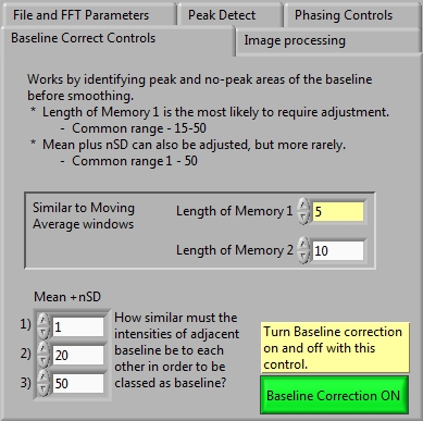
Figure 8: Baseline Correct Controls.
- Length of memory 1– similar to a moving average window
- Is the initial decimation length
- Length of memory two
- Baseline smoothing decimation length
- Mean + nSD
- Acceptance criteria for a point being in the baseline
- Baseline Correction ON/OFF
- Toggles baseline correction function on and off.
In general, these values are unlikely to need a great deal of adjustment except when changing between very different samples. Length of memory 1 is the most likely to need changing.
7.5 Identify initial region
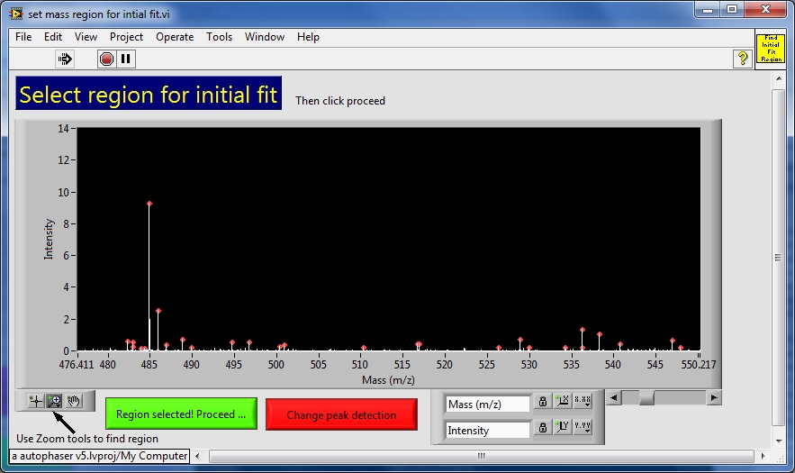
Figure 9: Select initial region user interface.
If there are not enough detected peaks in your initial fit region, you will be prompted to select an intial region.
You can either:
- Use the graph zoom tools to select you region of choice
- Type directly into the x axis (on the largest and smallest numbers)
- The length of initial region should be varied depending on the starting mass - larger masses can use larger initial regions. For estimates on the approximate length to use across the mass range, see the table in Section 7.3.
Then hit the “Region selected!” button ton continue.
Or, hit the “Change peak detection” button to redefine your peak detection parameters.
8 Peak Detection window
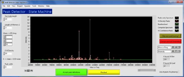
Figure 10: Peak detection user interface.
Use this window to tune the peak detection settings for the current spectrum. You can access the same controls as can be found on the Autophaser front panel, but now you can also see the spectrum and the detected peaks. See the Peak Detect Section 6.2 above for more information on the main peak detection controls. Other controls are:
- Accept peak definitions - to accept the peak definitions and continue.
- Change spectral Parameters – to return to the Autophaser front panel to, for example, change the mass range within which to search.
- Use all peaks for phasing – sometimes it will be necessary to use all peaks for phasing, rather than just the most intense peaks in a spectral region. This function can be controlled with this checkbox. This function will only rarely be necessary.
- Spectrum – standard Labview graph controls apply.
9 Brute force initial fit
The Fit Initial Region – Brute Force function takes all the peaks in the initial fit region and attempts to find a correction function for these points by a brute force method.
The phase correction function will have a quadratic relationship to the ICR frequency (for a spectrum recorded with a linear frequency sweep excitation or stored waveform inverse Fourier transform (SWIFT) excitation with a quadratic phase shift function4), and any quadratic function can be minimally defined by three points. Therefore, candidate phase correction functions for this initial region are generated by automatically selecting three peaks across the region: the largest detected peak (in magnitude mode) in the first, middle and last sections of the spectral portion. The first of these peaks is set to a relative phase wrap, n0, = 0. Values for the other two peaks (n1 and n2) are then scanned through available integer values of n between 0 and 2000. This range for n was empirically determined on data recorded on a number of different FT-ICR MS instruments. A wider range may be needed on other instruments. It should be noted that this method uses a least squares fitting approach and so obviously requires that there be at least three peaks in the initial region.
For each automatically generated value of ni, the corresponding correction values of φi are calculated according to the relationship:
|
|
|
(2) |
For each set of ni, least squares fitting is used to solve for a quadratic relationship (Eqn (12)) between frequency and phase shift and values of a,b and c are produced. From these values, the relative phase shift for all peaks in the region can be calculated and this information is used to calculate an absorption mode amplitude for each peak. A figure of merit for the quality of this trial phase correction function can be produced using the following method.
With the correct phase correction function (derived from the phase wrap values assigned to the three selected peaks), the intensity of all peaks in the initial test region (discounting harmonic peaks and those from external noise) in the absorption mode spectrum would be maximised. Therefore, in order to understand the quality or success of the phase correction function, a Figure of Merit (FoM) is calculated for each peak expressing the accuracy of the phase correction:
|
|
|
(3) |
The total FoM (FoMTotal) for a given phase correction function, for a spectrum or part of a spectrum containing N peaks is:
|
|
|
(4) |
This FoMTotal is recorded (based on all peaks in the initial region) for all tested combinations of ni for the three test peaks, and the combination which results in the highest FoMTotal is used to define the initial phase correction function that is passed onto the next section of the Autophaser algorithm. If no distinct maximum is found then this may indicate that the initial region used was too wide and the relative phase shift across that region exceeded 2000 cycles, or that the region contained a large proportion of low intensity peaks for which spectral noise had degraded the quality of the peak definition (peak maximum frequency and phase). So, the user must either reduce the length of the initial region to assess whether the relative phase shift was too great or adjust the parameters of the peak detection to avoid including poor signal-to-noise peaks.
In the absence of any other information, fitting to the initial region would require four million calculations (n can be any integer value between 0 and 2000 for two peaks, hence the total number of combinations of ni for the three peaks is 20002). However, it is possible to dramatically reduce the numbers of possible valid combinations of ni for all three peaks because it is known that although the phase correction function is quadratic, the function is actually very close to being a straight line, over a small mass range. Therefore, with n1 for the first peak held at zero, n2 for the second peak set at a known value (between 0 and 2000), and the frequency of all three peaks known, linear extrapolation can be used from the first two peaks to define a relatively small potential range of n3 for the last peak (usually a range of ±5, around the linear extrapolation of points n1 and n2 at the frequency corresponding to n3). In practice, this method of predicting a small range of values of n3 for the third peak, for every loop, reduces the total number of calculations done in the initial fitting region by two to three orders of magnitude.
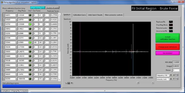
Figure 11: Fit initial region user interface.
The peak frequencies and phases of all the peaks in the initial region and shown in the table to the left hand side of the user interface. The three peaks being used for the fitting are those with “Use?”=T. This table can be used to manually attempt to solve the correction function for the initial region in a manner similar to that described by Qi et al. This information can be provided on request.
The display tabs show most of the important results:
- Spectrum tab
- Spectrum – shows the product of using the current phase correction function to produce an absorption mode spectrum. The original absorption mode (uncorrected) and magnitude mode spectra are also displayed for comparison.
- Accept calibration function – hit to accept the current phase correction function.
- Change peak definitions – hit to change the peak definitions.
- Use Wobbler – is turned on, uses the current tuning function to try to further tune the phase correction function.
- Calibration tab
- Shows the current calibration curve – toggle between showing just the 3 selected peaks and all peaks using the button called “Just selected peaks” in the UI window above.
- Initial search results
-
-
- This tab shows the summed FoMs for all the candidate phase correction functions which were searched. In the example below, you can see that there is a clear maximum value for the best candidate correction function.
-
-
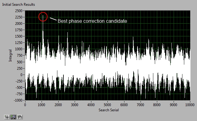
Figure 12: Highlighting a distinct maximum in the initial search results.
If you do not see such a clear maximum value then it is unlikely that the phase correction function will be any good. Under such circumstances, it may be necessary to change the peak detection parameters or change the initial fit region (which usually means making it shorter – try reducing it to 75% of its current length and repeat). Alternatively, change to a different initial region entirely.
10 General Comments
Autophaser is only a developmental programme and so will almost certainly contain bugs and annoyances. It is provided as is, and although we will endeavour to provide updates as we can, we do not have the capabilities to produce professional software or support yet. Therefore please excuse any rough edges.
If you realise that the programme will take a long time to process a file using a particular set up, you can simply restart it to get it to go again.
Very low signal to noise spectra, or those where the majority of peaks have low signal to noise, may not phase successfully. This may be because the noise component of the phase values of the peaks means that it is not possible to get a good estimation of the peak phase meaning that it is impossible to optimise the phase correction function adequately.
10.1 Mass calibration
The mass calibration used in the Bruker file formats will be the external mass calibration only. We have to been able to find a simple way to crack into the internal calibration functions on the Bruker data-files – particularly as this format has changed recently, to a largely binary format. Therefore, the absorption mode spectrum will require recalibration in Bruker DataAnalysis software before it can be compared to the results from the magnitude mode spectrum.
11 Example data file
An example data file can be uploaded from here. This file contains a Bruker .d format file of the FT-ICR MS spectrum of a sample of Guinness and a set of example phasing parameters (the *.ppf file) which can be used for phase correcting the data file.
To load the data file, use the browse button next to the File path control on the "File and FFT Parameters" control tab to navigate to the location where you unzipped the Guinness data file. As the file is a Bruker .d file, this is actually a folder, so to select that folder, double click it to open it and then click "Select current folder".
Now, load the phasing parameters wil by clicking the "Load parameters" button, also on the "File and FFT Parameters" control tab. Navigate to the *.ppf file that was also unzipped. This should load the phasing parameters file.
Now, you can hit "Begin".
Once this file has phased once, you can then go back and see what happens when you adjust, for example, some of the peak detection parameters.
12 Phasing of Images
To phase a complete image, or part of an image, select (File path control, File and FFT tab) a pixel from the image which is representative of the image. This pixel is known as the "Core" pixel. Use the normal method of single spectrum phase correction to phase correct this pixel. Now move to the Image Processing Tab.
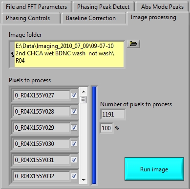
On the image processing tab, use the Image folder control to navigate to the folder which contains the spectra of all the individual image pixels. This will contain a list of folders of the type 0_R0nXxxxYyyy.
Once the correct folder has been selected, click "Run Image".
This will bring up the "Choose Image Section" window.
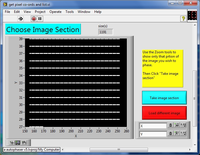
The Choose Image Section window shows a point at the coordinates of every pixel in the image. Use the zoom tools to identify the section of the image you wish to phase correct to absorption mode. Then click "Take image section".
To phase the complete image - just zoom out to the entire image.
To select another image, click the "Load different image" button.
Once the "Take image section" button has been clicked, this will start Autophaser processing the image. It will load the "Core" pixel and phase this again. Importantly, Auto-phaser will use the peak detection threshold for the core pixel and will apply this to all other pixels. It will also use the phase correction function for the core pixel as the basis for all pixels - although each pixel will be optimised individually.
The progress of the image processing can be tracked on both the "Image processing" controls tab and on the "Image Processing" display tab.
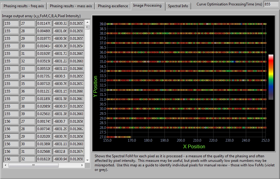
The Image Processing display tab has two indicators. The "Image output array" contains the information that will be saved in the .pip (phased image parameters) file. This file holds the phase correction information for each phased pixel and is designed to be read by the AMOLF MSI Datacube processing software. When this is released, it will allow the user to create absorption mode FT images.
The graph indicator shows informaiton allowing the user to track the phase correction sucess of each pixel. The colour of the square indicates how well Autophaser believes it has phase corrected each pixel, based on the average FoM of all peaks in the pixel. THe colour scale goes from Grey (poorest quality phasing in the image) to white (highest quality of phasing). This output can be used to target the user's attention onto specific pixels which are poorly phased, relative to other pixels in the image. This FoM information is also stored in the .pip file in column 2.
13 Reference list
(1) Williams, B.; Cornett, S.; Dawant, B.; Crecelius, A.; Bodenheimer, B.; Caprioli, R. in Proceedings of the 43rd annual Southeast regional conference - Volume 1. ACM: Kennesaw, Georgia, 2005, pp 137-142.
(2) Friedman, J. A Variable Span Smoother; Technical Report 5. Laboratory for Computational Statistics, Dept. of Statistics, Stanford University: Stanford, 1984.
(3) Savitzky, A.; Golay, M. J. E. Anal. Chem. 1964, 36, 1627-1639.
(4) Xiang, X.; Grosshans, P. B.; Marshall, A. G. Int. J. Mass Spectrom. Ion Processes 1993, 125, 33-43.