Public Policy
In our model the probability of school not becoming infected between
is given by
this is equivalent to a time-inhomogeneous poisson point process with rate
. This allows us to interpret
as an infectious pressure. We may compute a schools expected infectious pressure in the usual way:
We consider this over all time in order to make sure the pressures are comparable. The summarize for the values of are shown in the next table:
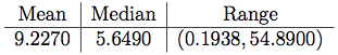
The idea of this policy consists on closing those schools with highest values for for the whole epidemic period.
We decide to close those schools with values higher than the 90% quantile and get the following results
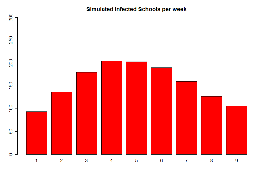
Since, the results are basically the same as in the actual simulation, at most we avoid the infection spreding around 40 schools, apart from the 37 schools that were closed. We decide to analyse other options.
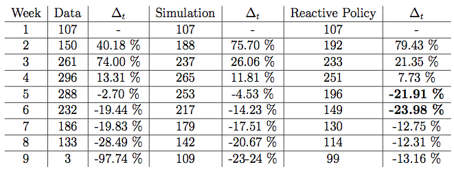
The second idea, consists on a reactive policy, which seems more natural. Now, once we detect an infected school we closed for the expected value of their infectious period, which in our case is 4 weeks. The results are as follows:
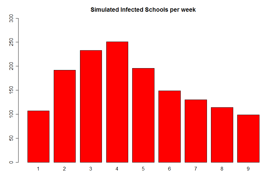 Here we can appreciate a consider improvement on the drop-off of infectiious schools through time, since now the higher percentage of recovery is achieved on week five rather than on the later weeks as in our actual simulation. This fact is ilustrated on the following table, were
 represents the increase / decrese in the amount of infected schools at time
compared with time
.