Atomistic / Nonlinear Elasticity Coupling Model

In The Exterior Domain

One model used to approximate atomistic systems is the following. We divide the lattice into two parts: $\Omega^a$ and $\Omega^c$ . We retain the atomistic properties of the system in $\Omega^a$ , but in $\Omega^c$ we replace atoms by a continuum which is deformed according a law of nonlinear elasticity derived from the potential the atoms interact by. We apply the Cauchy Born Rule: for a displacement field $u$ the Cauchy Born energy of the deformation is given in general by

$\mathcal{E}(u)= \int W(\nabla u) dx,$

where $W$ is the stored energy density. In our case, this is given by

$W(F) = \det A \cdot V(F \cdot R)$

where $V$ is the atomistic potential, $R$ the interaction range and $A$ is the determinant of the matrix that specifies the lattice in $\mathbb{Z}^2$ - which for us is the identity.

Lastly we must couple the two systems together: by adding in a continuum region, a problem is encountered on the boundary. The atoms there only have a part of the difference stencil needed to ascribe them a potential. For technical reasons, it is preferable to construct enough atoms to define a potential on these atoms, by only using data in the atomistic region. A discussion of this topic can be found here.

For practical purposes we must use the finite element method to minimise the energy of a function defined on a triangluation of the atomistic region. This can be coarse grained to reduce complexity, but we have not done this.

At The Interface

We use a particular method of reconstruction called the Geometric Reconstruction Atomistic Coupling (GRAC), which allows for a consistent coupling between these two regimes, and absent of spurious 'ghost forces' in the case of uniform deformations, a desirable trait. These forces arise due to the longer range atomistic potentials that impose forces on the continuum, due to the localised nature of the Cauchy Born model, it can not balance these longer forces and we would be left with a permanent imbalance error in the model. Below shows an image of the GRAC model

GRAC

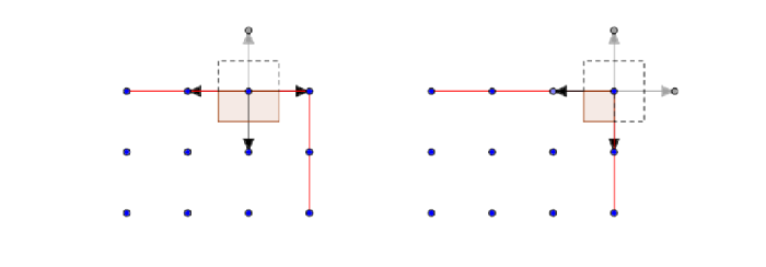
The solution proposed with GRAC is to modify the potential on the interface nodes $\Lambda^i$ . Firstly the atoms are given a effective volume, this is based on the proportion of the atomistic energy contribution relative to the continuum energy contribution outside the atomistic domain in the voronoi cell of the atom. in a square domain for example this will have value 1/2 on and edge, 1/4 for a corner.

Secondly we modify the site energy functional on $\Lambda^i$ (recall our atomistic domain $\Lambda^{a,i}=\Lambda^a \cup\Lambda^i$ interior and interface subdomains of our lattice), such that it gives a natural value to the 'missing' gray differences seen in above figure
$\Phi^i_l(y) := \sum_{j=1}^4 V(\tilde{D}_1y(l), \tilde{D}_2y(l), \tilde{D}_3y(l), \tilde{D}_4y(l))$

Where $\tilde{D_iy}=D_iy$ on all sides of the domain but the $i^\text{th}$ , and on that side it is the reflection of the bond 'opposite', i.e $D_iy = -D_{-i}y$ . On the diagram, the gray arrows take value of the opposite black arrow reflected.

In this way we have defined (for convenience reference deformation is 0):

$\mathcal{E}^\text{GRAC}(u) = \sum_{\ell \in \Lambda^i} w^i_l (\Phi^i_l(u) )\hspace{20pt} \text{where } w^i_l = \begin{cases} \frac{1}{2} &\text{if $\ell$ is an edge atom} \\ \frac{1}{4} &\text{if $\ell$ is a corner atom} \end{cases}$

We then search for displacements that will minimise the combined energy functional

$\mathcal{E}^{ac}(u)= \mathcal{E}^a(u) + \mathcal{E}^\text{GRAC}(u)+\mathcal{E}^c(u)$

Consistency and Convergence Rates

We are interested in comparing our models effectiveness compared to that of the pure atomistic model over the theoretical domain. Error estimates rely on convergence rates determined by studying the consistency of our model: coupled with (assumed) stability of the coupled model, we can acquire a priori estimates on the convergence rates of our numerical scheme. For the exact model, we have that

$\langle \delta \mathcal{E}^a(u) \rangle = 0 \; \forall v \in \dot{\mathscr{W}_h}^{\text{ac}}$ .

By consistency of a model, we mean that

$\langle \delta \mathcal{E}^{ac}(u) ,v\rangle = \gamma_{cons} \; \forall v \in \dot{\mathscr{W}}^{1,2}.$

for some small $\gamma$ : In fact, this will depend on the size of the domain we use the exact atomistic description in. The consistency error is then

$\langle \delta \mathcal{E}^{ac}(u)- \mathca^l{a}(u),v \rangle$

In order to obtain estimates, it is advantageous to write every component of the consistency error in the same way: we ask if

$\langle \delta \mathcal{E}^{ac}(u), v \rangle =? \sum_{edges} \eta^{ac}_e D_ev$ .

If we can find such a representation, we can evaluate the consistency error directly: it is of course a simple matter to write the atomistic energy variation in terms of bonds, for this is what the potentials are really defined on. To do this, we will discretize our domain using Q1 finite elemets- we pick a square mesh whose nodes lie exactly on atomistic positions, for simplicity.

There are 3 terms to bound: we have $\mathcal{E}^{ac}=\mathcal{E}^a(u)+\mathcal{E}^i(u)+\mathcal{E}^c(u)$ with these energies defined on disjoint regions. We must restrict the exact energy to these regions to perform calculations. This makes the first term easy! Our method is of course consistent in the atomistic region, because we use this exact description there.

There are then 2 more terms to deal with: the interfacial consistency error and the continuum region error. It is helpful to look at the 'boundary' of the continuum region seperately: that is, the Q1 elements that share an edge with the atomistic region.

For the interior of the continuum region, we can write

$\int_{\Omega_c}\nabla W(\nabla u) \cdot \nabla v &= \sum_{Q \in \Omega^c} \int_{Q}(\nabla W(\nabla u) -\nabla W(F_Q)) \cdot \nabla v +\sum_Q\nabla W(F_Q)\int_{Q} \cdot \nabla v$

$\leq R^{-3}||\nabla v||_{L^2} +\sum_{Q \in \Omega^c} \int_{Q}\nabla W(F_Q) \cdot \nabla v$

with R the radius of the atomistic region, and $W_Q$ the average gradient of $u$ in each tile. In doing so, because we have Q1 test functions the final integral can be evaluated exactly. We also have the decay rates of the exact solution from this paper.By calculating the derivatives for the Cauchy Born strain, we arrive at the following:

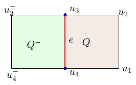
$\sum_{e \in \Omega_c} \eta^{ac} D_ev = \sum_{e \in \Omega_c} (f'(F^{Q^{-}}_{e})+f'(F_{e}))D_ev, \; \; \text{F defined on each Q}.$

continuum tile

For instance, the difference on the edge e is $D_eu = u_3-u_4$ . By expressing all these terms as above and performing taylor expansions, we can bound the consistency error:

$\left(\sum_{e \in \text{int}(\Omega^c)}(\eta_e^{ac}(u) -\eta^a(u))^2\right)^{\frac{1}{2}}&\leq 4C\left(\sum_{\ell \in \text{int}( \Omega^c)}|D^3u(\ell)|^2\right)^{\frac{1}{2}} \leq C\left(\sum_{\ell \in \text{int} (\Omega^c)}|\ell|^{-8}\right)^{\frac{1}{2}}$

$\approx C\left(\int_R^{\infty} r \cdot r^{-8} dr\right)^{\frac{1}{2}} =\frac{C}{R^{\frac{6}{2}}} =\frac{C}{R^3}.$

On the boundary of the atomistic and continuum region we only have 1 tile contribute to the consistency calculation: but from above, we also only have half the atomistic weighting due to the GRAC coupling also being subtracted. We can only extract the following rate:

$f'(D_eu) -f'(F_e^{Q}) &\approx \frac{C}{2}\left((u_4-u_1)-\frac{(u_3-u_2)+(u_4-u_1)}{2}\right) =\frac{C}{2}\left((u_4-u_1)-(u_3-u_2)\right)$
$\lesssim \frac{1}{\ell^2} - \frac{1}{(\ell+1)^2} \lesssim \frac{2\ell +1}{\ell^4} \lesssim \frac{1}{\ell^{-3}},$

$\sum_{e \in \mathscr{E}^i}(\eta_e^{ac}(u) -\eta^a(u))^2 \lesssim \left( \int \frac{1}{R^6} dl\right)^{\frac{1}{2}} \lesssim \left(\frac{R}{R^6}\right)^{\frac{1}{2}} \lesssim R^{-\frac{5}{2}}.$

showing that the boundary is the biggest source of error in the above model.

an graph

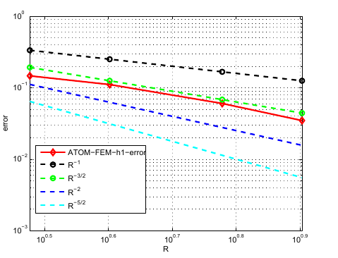
Numerical results show that we can get at least a rate of $R^{-2}$ : it is difficult to run sufficently large simulations to test our implementation. The above graph was produced by using a very large atomistic grid as a 'reference solution' to base the error calculations from.