
Approximate Bayesian Calculation
Brief on ABC
Approximate Bayesian Computation (ABC) aims to tackle problems with intractable likelihood by approximating the posterior distribution without explicit likelihood evaluation. The original ABC rejection sampling algorithm is as follows, as presented in Beaumont (2002).
- Propose \( \theta_0 \) from prior \( p(\theta) \).
- Compute \( S_{\theta_0} \)
- For \( U \sim U(0,1) \), accept \( \theta \)
Suppose \( \theta \) is an unknown parameter of interest with prior \( \pi( \theta) \) . The algorithm proposes values \( \theta_0 \) from the prior, and accepts them with some probability. Suppose \( S \) is a summary statistic computed from a data set, and let \( D \) be the observed value of this summary statistic given the value \( \theta_0 \).
Instead of considering the full likelihood, we now accept proposals with probability proportional to \( \mathbb{ P }( S = D | \theta ) \), that is the proposal \( \theta \) is accepted if
\begin{equation*}
\mathbb{ P }\left( S = D | \theta \right) > \max_{ \theta' \in \Theta }\left\{ \mathbb{ P }\left( S = D | \theta' \right) \right\} U
\end{equation*}
where \(U \) is an independent random variable with distribution \( U \sim U(0,1) \). It can be shown that when \(S \) is a sufficient statistic for \( \theta \) the algorithm results in a sample from the posterior distribution.
The algorithm suffers from two main drawbacks:
- Firstly, it can be very difficult to evaluate \( \mathbb{ P }\left( S = D | \theta \right)\) in practice.
- Secondly, \( \mathbb{ P }\left( S = D | \theta \right) \) can be very small (even 0 in the case of continuous distributions), resulting in very few accepted proposals.
Instead of considering \( \mathbb{ P }\left( S = D | \theta \right) \) directly, simulate a sample from the model under \( \theta \), compute the summary statistic from the simulated data set (denoted \(D_S \)) and consider accept proposals when \( D_S = D \). This approach overcomes the first problem by removing the need to calculate probabilities explicitly, but still suffers from the second problem since in most situations \( \mathbb{ P }\left( D_S = D | \theta \right) \) will be very small even for plausible values of \( \theta \).
The second problem problem can be overcome by introducing a tolerance \( \epsilon > 0 \) , and accepting a proposal whenever \( || D_S - D || \leq \epsilon \) in some appropriate norm.
The value of \( \epsilon \) will have to be fine-tuned on a case-by-case basis, but if an appropriate tolerance can be found then the second problem is also resolved.
ABC for the SLFV
Implementing ABC for the SLFV model requires specification of a test statistic. A sufficient statistic ensures that a sample generated by ABC is from the exact posterior distribution, provided \( \epsilon \)= 0 (see Beaumont 2002). Unfortunately, there are no known sufficient statistics for the Fleming-Viot process in general, but Tavare (1997) argues that many statistics are suitable for practical inference.
We use an approach which measures homogeneity in the lineages in the sample. To make this precise, we divide the sample of n lineages into \( \lfloor n/2 \rfloor =: n_0\) disjoint pairs. We label these draws as \((d_i, m_i )_{ i = 1 }^{ n_0 }\), where \(d_i\) denotes the euclidean distance between the \(i^{ \text{th} }\) pair and similarity score \(m_i\) given by for a pair \((x_{i_1}, x_{i_2})\):
\begin{equation*}
m_i :=
\begin{cases}
1 &\text{ if } \kappa^{ ( i_1 ) } = \kappa^{ ( i_2 ) } \\
0 &\text{ otherwise}
\end{cases}
\end{equation*}
It remains to specify how to pair the individuals. Choosing pairs to cover a wide range of distances is a good approach, which we achieve in a cheap way by pairing individuals uniformly at random.
In order to simulate similar binary vectors \(\mathbf{m}^{\theta}\) from the SLFV model we derive the probability of identity, \(\psi_{ \theta }(x)\) of two individuals sampled at separation \(x\) as follows.
\begin{align*}
0 = &( 1 - \psi_{ \theta }( x ) ) \psi_{ \theta }( x ) \int_{ 0 }^{ \infty } | B_x( r ) \cap B_0( r ) | \int_0^1 u^2 \nu_r( du ) \mu(dr ) \\
&+ \int_{ \mathbb{ T } } \int_0^{ \infty } \int_0^1 \frac{ 2u }{ \pi r^2 } ( | B_0( r ) \cap B_y( r ) | - u | B_0( r ) \cap B_y( r ) \cap B_x( r ) | ) ( \psi_{ \theta }( x - y ) - \psi_{ \theta }( x ) ) \nu_r( du ) \mu( dr ) dy \\
&- 2m \psi_{ \theta }( x ) \left( \psi_{ \theta }( x ) - \psi_{ \theta }( x ) Q_1(d,P) + ( \psi_{ \theta }( x ) - 1 ) Q_2(d,P) \right)
\end{align*}
We then would numerically solve this non-linear equation in order to get numerical values for the probability of identity.
A degree of freedom to consider is how to pair the original individuals. It would seem that choosing pairs to cover a wide range of distances is a good approach, but for our initial trials we just choose the pairs uniformly at random over the spatial region.
The following algorithm will provide a value \( \theta\), approximately from the desired distribution given the observed data \( \pi( \theta | \eta) \).
ABC Algorithm using Pairing Statistic
Inference Results
Using the previous algorithm, ABC was performed on a sample of size 10,000 of two different types, in a torus of side length \(L=10\), assuming a mutation rate \( \theta=0.05 \) and using a uniform prior on the interval (0,0.1).
In addition, different values for \( \epsilon \) were tested in order to have some idea of the sensitivity of the approximate likelihood to this variable. Similarly, different refinements for the mesh used in the numerical scheme were tested.
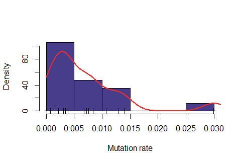
Below: Likelihood function using length interval h=2 for the mesh and \( \epsilon=47\% \).
 Below: Likelihood function using length interval h=2 for the mesh and \( \epsilon=48\% \).
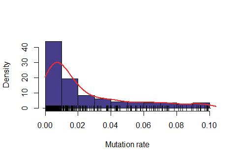 Below: Likelihood function using length interval h=2 for the mesh and \( \epsilon=50\%\).
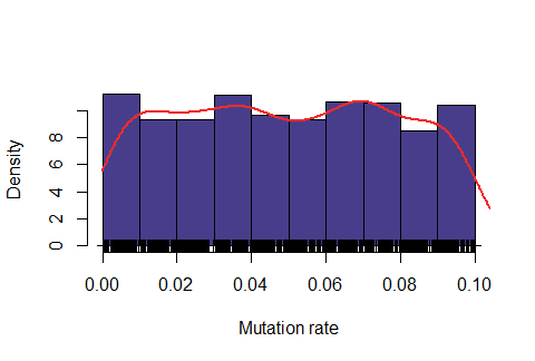
Observe that the likelihood is actually "too" sensitive to the value of \( \epsilon\). For \(\epsilon=47\%\), most of values were rejected, for \(\epsilon=50\%\) almost all values were accepted and for \(\epsilon=48\%\) it seems to produce a feasible likelihood. In addition, the computing time is also quite dependent on this variable. For \(\epsilon=47\%\), on average it took around 6.5 minutes for obtaining one accepted value, for \(\epsilon=48\%\) around 1.1 minutes and for \(\epsilon=50\%\) around 0.2 minutes.