
Stochastic Volatility Models
In the previous sections we have only considered price processes where the coefficients in the governing SDE are constant (see section on jump-diffusion models). One can also consider models where the coefficients are functions of time and the stock price.
An alternative approach is to allow the paremeters such as the volatility \(\sigma\) to be random variables themselves. More precisely, we look at models of the form \((Y_t, V_t)\) where the log-price \(Y_t\) and the volatility \(V_t\) are governed by different SDEs. These type of models are often called stochastic volatility models and an example of which is the Barndorff-Nielson--Shephard (BNS) model. The BNS model is of the form
\(\begin{align} \mathrm{d}Y_t &= \Big(r -\delta - \frac{1}{2}V_t\Big)\mathrm{d}t + \sqrt{V_t}\mathrm{d}W_t + \rho\mathrm{d}J_{\lambda t}, \\ \mathrm{d}V_t &= -\lambda V_t \mathrm{d}t + \mathrm{d}J_{\lambda t}, \end{align}\)
where \(r,\lambda>0\), \(\rho<0\), \((W_t)_{t\geq 0}\) is a standard Brownian motion and \((J_{\lambda t})_{t\geq 0}\) is a pure jump process that increases almost surely and has Levy measure \(\nu\). \(\delta\) is a time-independent constant which is chosen so that the discounted asset price \(\tilde{S}_t = \exp(-rt + Y_t)\) is a martingale. It can be shown that necessarily \(\delta = \lambda\kappa(\rho)\) where \(\kappa\) is the cumulant generating function of \((J_t)_{t\geq 0}\) given by
\( \kappa(u) = \int_0^\infty (e^{u\xi} - 1) \;\nu(\mathrm{d}\xi). \)
The negative constant \(\rho\) is there to introduce a correlation between the log-price and the volatility; a jump in the volatility will cause a jump downwards in the log-price. Typically, the jump term \((J_t)_{t\geq 0}\) is taken to be a compound Poisson process
\( J_t = \sum_{i=1}^{N_t} U_i \)
where \( (N_t)_{t\geq 0} \) is a Poisson process with intensity \(\alpha\) and \(\{U_i\}_{i\in\mathbb{N}}\) is a sequence of i.i.d. random variables which we assume to be exponentially distributed with mean \(1/\eta\) and so \(J_{\lambda t}\) has Levy measure given by \(\nu(\mathrm{d}h) = \alpha\lambda g(h)\) with \(g(h) = \eta\exp(-\eta h)\) being the density of a exponentially distributed random variable. For this choice of \( (J_t)_{t\geq 0}\) a simple integration shows that
\(\kappa(\rho) = \frac{\alpha \rho}{\eta - \rho}\).
As before option prices are given as expectations of the payoff under the risk neutral measure so Monte Carlo methods can be used.Notice that the BNS model is a two-dimensional model so one needs to approximate it by a Markov chain on a finite two-dimensional state space. In one-dimensional models the Q-matrix \(\Lambda\) of the approximating chain is a \(N\times N\) matrix where \(N\) is the number of grid points. If now we have \(N\) grid points in bothe the log-price and the volatility component then the Q-matrix is a \(N^2\times N^2\) matrix. Thus, simulations of these higher dimensional models can be computationally expensive.
As in the jump-diffusion case we calculate the Q-matrix of the Markov chain by considering the jump and the diffusion components of the process separate and compute the corresponding transition rate matrices \(\Lambda_J\) and \(\Lambda_D\), then \(\Lambda\) is defined as the sum \(\Lambda\) = \(\Lambda_D + \Lambda_J\).
Diffusion Matrix
We can express the diffusion part of the BNS model in vector form as
\(\mathrm{d}\begin{pmatrix} Y_t \\ V_t \end{pmatrix} = \begin{pmatrix} r- \delta - \frac{1}{2}V_t \\ -\lambda V_t \end{pmatrix}\mathrm{d}t + \begin{pmatrix} \sqrt{V_t} \\ 0 \end{pmatrix}\mathrm{d}W_t\)
which provides the infinitesimal generator \(\mathcal{L}_D\) as
\(\mathcal{L}_Df(y,v) = \Big(r - \delta - \frac{1}{2}v\Big)\frac{\partial f}{\partial y}(y,v) - \lambda v\frac{\partial f}{\partial v}(y,v) + \frac{1}{2}v\frac{\partial^2 f}{\partial y^2}(y,v).\)
where \(f \in C_0^2 (\mathbb R ^2)\) the space of twice differentiable functions such that \(\lim_{|x|\to\infty}f(x) = 0 \). One can discretize this PDE by finite differences using either forward or backward difference for the first order derivatives:
\(\frac{1}{h}\Big( f(y + h,v) - f(y,v)\Big)\quad\text{or}\quad \frac{1}{h}\Big( f(y,v) - f(y - h, v)\Big)\)
The choice of which one to use is determined by the condition that the result must be a Q-matrix. For the second order derivative term central difference can be used:
\(\frac{1}{h^2}\Big( f(y + h, v) - 2f(y,v) + f(y - h,v)\Big)\).
The forward, backward and central differences in the \(v\) variable are defined similarly. Let \(\mathbb{G} = \{(y_i,v_j) : 1\leq i,j\leq N, y_1 > \cdots > y_N, v_1 < \cdots < v_N\}\) be a grid with grid spacing \(h_v\) in the volatility component and grid spacing \(h_y = |\rho|h_v\) in the log-price component. The choice of the grid spacing \(h_y\) is so that a jump in the volatility of one grid point translates to a jump of one grid point in the log-price and so on. Now denote \(f(y_i,v_j)\) by \(f_{ij}\) then the discretisation of \(\Lambda_D\) is
\(\frac{1}{h_y}\Big(\mu f_{i-1j} - \mu f_{ij} - \frac{1}{2}v_jf_{ij} + \frac{1}{2}v_jf_{i+1}j\Big) + \frac{1}{h_v}\Big(\lambda v_jf_{ij-1} - \lambda v_jf_{ij}\Big) + \frac{1}{h_y^2}\Big(\frac{1}{2}v_jf_{i-1j} - v_jf_{ij} + \frac{1}{2}v_jf_{i+1j}\Big)\)
It is easy to see that the above equation can be expressed as a matrix-vector product \(\Lambda_J \mathbf{f}\) where \( \mathbf{f} = \big(f_{11},f_{12},\ldots,f_{1N},f_{21},\ldots,f_{NN}\big)^T \) and the \(\Lambda_J\) is the desired discretisation.
Jump Matrix
In general, the generator of a compound Poisson process on \(\mathbb{R}^d\) is given by
\( \mathcal{L}_J f(x) = \int_{\mathbb{R}^d} \big(f(x+h) - f(x)\big)\;\nu(\mathrm{d}h) \),
where \(f \in C_0(\mathbb{R}^d)\). In the BNS model, since the log-price process and the volatility are both driven by the same jump process with correlation \(\rho < 0\) we can write the generator \(\mathcal{L}_J\) for the jump component as
\(\mathcal{L}_Jf(y,v) = \int_{\mathbb{R}} \big( f(y + \rho h, v + h) - f(y,v) \big)\;\nu(\mathrm{d}h),\)
The above integral can be approximated by Riemann sums on the grid \(\mathbb{G}\),
\(\begin{align*}\mathcal{L}_J f(y_i,v_j) &\approx \sum_{n=1}^{N - (i\vee j)} \Big( f(y_i + n\rho h_v,v_j + nh_v) - f(y_i,v_j) \Big) \alpha\lambda g(h_v)nh_v \\ &= \sum_{n=1}^{N - (i\vee j)} \Big( f(y_{i + n} ,v_{j + n}) - f(y_i,v_j) \Big) \alpha\lambda g(h_v)nh_v \end{align*}\).
Again the above can be written as a matrix-vector product \(\Lambda_J\mathbf{f}\) where \(\mathbf{f}\) is as above.
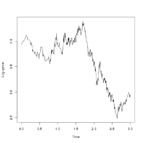
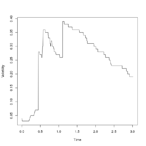
The above graphs show a sample path of the log-price and the volatility obtained from the approximating Markov chain. A grid of size 100 \(\times\) 100 was used to generate the path. Notice that the log-price looks like a typical jump-diffusion process while the volatility maoves up entirely by jumps and slowly drifts to zero in the abscence of jumps due to the negative term in the governing SDE.